Where does the ln come from in S = k ln(W) ? - Take 2

source

Some years ago I wrote this post. Now I want to come at it from a different angle.

A closed system spontaneously goes towards the state with maximum multiplicity, $W$. For a system with $N$ molecules with energies $\varepsilon_1, \varepsilon_2, \ldots $ we therefore want to find the values of $N_i$ that maximises $W(N_1, N_2, \ldots)$.

This is easier to do for $\ln W$ than $W$, which is fine because $W$ is a maximum when $\ln W$ is a maximum, and this happens when
$$ \frac{N_i}{N}= p_i = \frac{e^{-\beta \varepsilon_i}}{q} $$
$\beta$ can be found by comparison to experiment.  For example, the energy of an ideal monatomic gas with $N_A$ particles is
$$ U^{\mathrm{Trans}} = N_A \langle \varepsilon^{\mathrm{Trans}} \rangle = N_A\sum_i p_i \varepsilon_i = \frac{3N_A}{2\beta} = \tfrac{3}{2}RT \implies \beta = \frac{1}{kT} $$
where $R$ is determined by measuring the temperature increase due to adding a known amount of energy to the system.

So far we have used $\ln W$ instead of $W$ for convenience, but is there something special about $\ln W$? Yes, the change in $\ln W$ has can be expressed quite simply
$$ d \ln W = \beta \sum_i \varepsilon_i dN_i = N \beta \sum_i \varepsilon_i dp_i =  \frac{dU}{kT} $$
So change in internal energy $U$ due to a redistribution of molecules among energy levels is equal to the change in $\ln W$ (as opposed to $W$) multiplied by $kT$
$$ dU = Td\left( k \ln W \right) = TdS$$
The final question is whether there is something special about $\ln = \log_e$ as opposed to say $\log_a$ where $a \ne e$? Well, $\log_a W$ is a maximum when
$$ \frac{N_i}{N}= p_i = \frac{a^{-\beta \varepsilon_i}}{q} $$
There is an extra term in the derivation but that cancels out in the end.  So no change there.

What about $\beta$?  There are two changes.  The previous derivation of $U^{\mathrm{Trans}}$ relied on this relation (I'll drop the "Trans" label for the moment)
$$  \varepsilon_i e^{-\beta \varepsilon_i}  = - \frac{d }{d \beta} e^{-\beta \varepsilon_i} \implies \langle \varepsilon \rangle = - \frac{1}{q} \frac{dq}{d\beta} $$
which now becomes
$$  \varepsilon_i a^{-\beta \varepsilon_i}  = - \frac{1}{\ln(a)} \frac{d }{d \beta} a^{-\beta \varepsilon_i} \implies \langle \varepsilon \rangle = - \frac{1}{q \ln(a)} \frac{dq}{d\beta}$$
While $q$ has an extra $\ln (a)$ term, the derivative wrt $\beta$ is still the same and
$$ U^{\mathrm{Trans}} = N_A \langle \varepsilon^{\mathrm{Trans}} \rangle = N_A\sum_i p_i \varepsilon_i = \frac{3N_A}{2 \ln (a) \beta} = \tfrac{3}{2}RT \implies \beta = \frac{1}{\ln (a) kT} $$
So, $S = k \log_e W$ is special in the sense that the proportionality constant $k$ is the experimentally measured ideal gas constant divided by Avogadro's number.  In any other base we have to write either $S = k \ln (a) \log_a W$ where $k = R/N_A$ or $S = k^\prime \log_a W$ where $k^\prime = \ln(a)R/N_A$

Clearly, $S = k \log_e W$ is the most natural choice, and this is because $e$ is the (only) value of $a$ for which
$$ \frac{d}{dx} a^x = a^x $$
In fact that is one way to define what $e$ actually is.



This work is licensed under a Creative Commons Attribution 4.0

Notes on fugacity and activity

This is one of those "note to self" posts where I try to get my head around a concept, this time fugacity and activity for a gas.

$dG=Vdp-SdT \implies dG=Vdp \text{ if } dT=0$

$$G(p)=G^\circ+\int_{p^\circ}^{p}Vdp$$
If the gas is ideal, i.e. for one mole $V=RT/p$, then
$$G(p)=G^\circ+RT\int_{p^\circ}^{p}\frac{dp}{p}=G^\circ+RT\ln\frac{p}{p^\circ}$$
For $A\rightleftharpoons B$
$$G(p_B)-G(p_A)=0 \implies \frac{p_B}{p_A}=e^{-\Delta G^\circ/RT}$$
What about a real gas where $V\neq RT/p$?  We introduce the fugacity $(f)$ for which $V=RT/f$ so that
$$G(p)=G^\circ+RT\ln\frac{f}{p^\circ} \text{ and } \frac{f_B}{f_A}=e^{-\Delta G^\circ/RT}$$
To determine $f$:
$$\int_{p'}^{p} (V-V_{ideal})dp=RT\ln\left(\frac{f}{f'}\cdot \frac{p'}{p}\right) =  RT\ln\left(\frac{f}{p}\cdot \frac{p'}{f'}\right) $$
Gases approach ideality at low pressure: $f'/p'\rightarrow 1$ as $p\rightarrow 0$ so:
$$\ln\left(\frac{f}{p}\right)=\ln(\phi)=\frac{1}{RT}\int_{0}^{p} (V-V_{ideal})dp$$
So for sticky non-ideal gases for which $V<V_{ideal}$ the fugacity coefficient $\phi$ is less than 1.  So even though $V=RT/f$ don't confuse $f$ with $p_{ideal}: f<p<p_{ideal}$ for a given number of gas particles.

Finally the relationship between fugacity and activity ($a$) is
$$a=\frac{f}{p^\circ}$$.

This work is licensed under a Creative Commons Attribution 3.0 Unported License. 
  

Taking my thermodynamics course online

Readers of this blog will know I occasionally dabble with the flipped classroom/peer instruction approach in my teaching, and this year I finally went whole hog - to use an Iowan expression.

What I did (tl;dr)
This year I abandoned the textbook for my part of the course and replaced the material with videos and Powerpoint slides.  This allowed me to completely change the order I taught subjects in and introduce more of what I think are more relevant subjects.

Why I did it
Last year I had already flipped the classroom and used lecture periods almost exclusively on peer instruction questions based on the assigned reading.  Now that I was finally happy with how I was teaching, I started to realize that I was less happy with what I was teaching.

What one is teaching, and the order it is being taught in, is to a large extent dictated by the textbook one chooses.  We chose Dill's Molecular Driving Forces. Like most textbooks it's written for the instructor rather than the students: an excellent resource for people who already understand the subject.  And why not?  I am the customer after all.

Thermodynamics/statistical mechanics books are essentially physics books that go through the definition and derivation of key equations and concepts first and in great detail and treat the applications as more of an afterthought.  Example: I would argue that $K=e^{-\Delta G^\circ/RT}$ is a more useful equation than, say, $S=q_{rev}/T$ for the practicing chemist, yet most books will spend many more pages discussing the latter. And don't get me started on the Carnot cycle.

Redesigning the curriculum I had five guiding principles in mind:

1. The video shown at the beginning of this post.
2. Start with the most useful (a much less arbitrary term than important) topics to my students.
3. Let the homework problems dictate the material, not the other way around.
4. Reduce the load and spend more time on what you consider most useful.
5. Study test test test – test.

So, one of the first homework questions I wrote involves computing $\Delta G^\circ$ from a binding curve.  Then I wrote the corresponding lecture notes.  Since I introduced this topic early, I also get to use it again and again during the rest of the course, which increases retention.

Similarly, I was able to introduce problems involving the Molecular Calculator, because I could taylor the lectures accordingly.

How I did it
1.  The homework problems.  I rewrote all the homework problems from scratch. It's hard to describe how liberating (and relatively easy) it is to write exactly the problems you want knowing that everything you need by definition will be covered in lecture, exactly how you want it.

As in previous years I put the answer up in form of multiple choice on PeerWise.  Once an answer is selected the solution (copied from my Maple solution) is revealed.  Occasionally, I also supplied intermediate solutions to help guide the student and screen-casts showing how I solve the problem using Maple.

Finally, I the students some choice in the problems they want to solve.  For example, I told them they had to solve any six out of nine questions.  I made sure that the first six were relatively easy, but some of the remaining questions could be quite tricky.  Many students did all of them, and I got few complaints about the most difficult ones since the students themselves had chosen to work on them.

You can find the problem sets here.

2. The video-lectures.  I chose to make video-lectures because it was the fastest way to generate material.  The Powerpoint slides contain mainly equations and pictures and all the explanation is done verbally (remember: the students can rewind and repeat).  This is much quicker than writing everything down in detailed lecture notes.

I make normal Powerpoint slides and use ScreenFlow to record (PC users can use Camtasia). Another option would have been pen-casting but many of the figures were much too complicated to sketch and screen-casting made it easier to introduce videos, simulations, etc. However, if you have handwritten lecture notes you are happy with, this could be a good option.

Each video lecture is quite short (max 10 minutes) and most end with a question. I provide the Powerpoint slides - except the ones containing the answer - along with the videos.  The students have to watch between four and six videos before each two-hour "lecture" period

The editing features in ScreenFlow make it relatively easy to correct mistakes.  If you remember to pause briefly (also verbally) between each slide, then you only have to repeat one slides worth of material.

You can see the videos and slides here

3. "Reading"-quiz.  The students have to take an on-line quiz (no points) the evening before the day of the lecture (at the latest): one question per video that can be easily answered if one has watched the video (often a T/F question).  I do this for two reasons: (1) to make it clear that they must prepare for class since I am not going to repeat the material and (2) that they should pay attention while watching the videos.   The last question on each quiz is whether I should discuss something in more detail in class.

4. The "lecture" period.  During the 2 x 45 min "lecture" period I ask roughly 20 peer instruction questions.  Roughly ten are review questions on previous material and the remaining questions are on the new material.  I use Socrative for voting.  Most are conceptual questions designed with discussion in mind.  

What I learned so far
1. Making the slides and videos and questions is a lot of work.  Even considering I have taught this course many times and knew exactly what I wanted to do.  But ...

2. ... it is much, much faster than writing a textbook yourself. Constructing such a textbook-replacement for your course is a manageable task. And extremely liberating and satisfying.

3. We live in the age of Google (OK, I kinda knew this one already).  You don't need to include a table of dielectric constants or heats of formation in your teaching material.  Just give a few examples of finding this info with Google in one of the early videos.

4. Review is essential.  The data from in-class voting is clear: take a question that 95% of the class answered correctly and ask is a week later.  Half the class will get it wrong.  Research shows that many subject must be reviewed at least 3 times before it sticks.  Keep this in mind when designing your curriculum.  Most courses pack in way too much material.  Very little of it sticks.  See the video at the beginning of the post again.

5. Surprisingly (to me) many of the students take the "reading quiz" at the very last minute and probably wouldn't prepare for class if it wasn't for the reading quiz.

Example: 30 students took the exam.  For the September 30 lecture period, 24 students completed the "reading"-quiz.  Eight of them completed the quiz between 11 pm and midnight (the deadline).

OK. That's it, for now.  Now would be a good time to watch the video a third time.  You know, so it sticks.

More posts one statistical mechanics can be found here.

This work is licensed under a Creative Commons Attribution 3.0 Unported License. 

The entropy increases when things fall apart

The translational entropy dominates when bonds are broken
An entropy change has four contributions$$\Delta S^\circ=\Delta S^{Molecular}+\Delta S^{\circ,Translation}+\Delta S^{Rotation}+\Delta S^{Vibration}$$For reactions where bonds are broken $S^{\circ,Translation}$ usually dominates.

For example for the reaction $H_2 \rightarrow 2H$ the entropy changes at 25 $^\circ$C are:$$\Delta S^\circ = 11.6+100.1-12.8-0.0=98.9 \text{ J/molK}$$For breaking the hydrogen bond between two water molecules, $H_2O\cdot \cdot \cdot HOH\rightarrow 2H_2O$, the free energy energy contributions are$$\Delta S^\circ =0.0+136.2+9.3-66.0=79.4  \text{ J/molK}$$In both cases $\Delta S^\circ$ is positive because two particles have more entropy than one.

In many cases $\Delta S^\circ \approx \Delta S^{\circ,Translation}$ is a reasonable approximation.

Test: What happens to the standard entropy for this process

     

Peer instruction question on enthalpy

Is this an endo- or exothermic process?

         

Negative temperature: the equations

A recent Science paper entitled Negative Absolute Temperature for Motional Degrees of Freedom has generated a lot of discussion on the blogosphere (example) already.  This post is about the equations behind the concept of negative temperature.  The discussion and figure is taken out of chapter 12 of the excellent book Thermodynamic Driving Forces by Dill and Bromberg.

The thermodynamic definition of temperature is
$$dS=\frac{dU}{T}=\left(\frac{dS}{dU}\right)_{V,N}dU\Rightarrow\frac{1}{T}=\left(\frac{dS}{dU}\right)_{V,N}$$while the statistical mechanical definition of entropy is $$S=k\ln(W)$$

For a two-state system (Figure 12.1)$$\frac{1}{T}=k\left(\frac{d\ln(W)}{dn}\right)_{V,N} \left(\frac{dn}{dU}\right)$$The multiplicity term can be rewritten as $$\ln(W)=\ln\left(\frac{N!}{n!(N-n)!}\right)\approx-n\ln\left(\frac{n}{N}\right)-(N-n)\ln\left(\frac{N-n}{N}\right)$$where the last term used Stirling's approximation $x!\approx (x/e)^x$. The internal energy is given by$$U=n\varepsilon_0\Rightarrow\frac{dn}{dU}=\frac{1}{\varepsilon_0}$$so $T$ can be defined in terms of the fraction of molecules in the ground $(f_{ground}=n/N)$ and excited state $(f_{excited}=1-n/N)$ $$\frac{1}{T}=\frac{k}{\varepsilon_0}\ln\left(\frac{f_{ground}}{f_{excited}}\right) $$At equilibrium these fractions are determined by the Boltzmann distribution$$\frac{f_{ground}}{f_{excited}}=e^{\varepsilon_0/kT}>1$$This is the $T$ you measure with a thermometer and this $T$ can never be negative at equilibrium.  However, if you create a excited macrostate for which $f_{ground}/f_{excited}<1$ then the corresponding variable $T$ can indeed be negative.  As pointed out by Michael de Podesta this happens all the time in a laser.



This work (except the first figure which is © by Garland Science) is licensed under a Creative Commons Attribution 3.0 Unported License.

The enthalpy increases when bonds are broken

Enthalpy changes comes mainly from changes in bonding
An enthalpy change has four contributions$$\Delta H^\circ=\Delta E^{Molecular}+\Delta H^{\circ,Translation}+\Delta H^{Rotation}+\Delta H^{Vibration}$$The molecular energy $\Delta E^{Molecular}$ is associated with the electrons and nuclei, i.e. chemical and intermolecular bonding, and this is often the largest term.

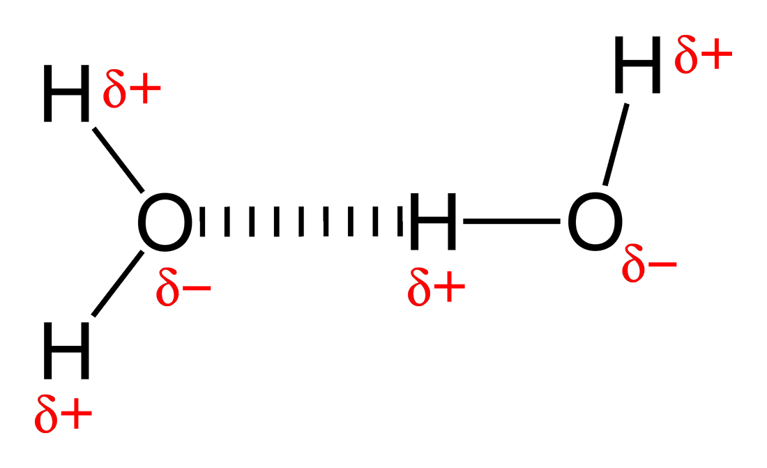
For example for the reaction $H_2 \rightarrow 2H$ the enthalpy contributions are:$$\Delta H^\circ = 460.2+6.3-2.5-26.4=437.6 \text{ kJ/mol}$$For breaking the hydrogen bond between two water molecules,$H_2O\cdot \cdot \cdot HOH\rightarrow 2H_2O$, the energy terms are$$\Delta H^\circ = 20.5+6.3+3.8-17.6=13.0 \text{ kJ/mol}$$In both cases $\Delta H^\circ$ is positive mainly because it requires energy to break a covalent bond or a hydrogen bond.

Figure 1. The attraction between partially charged atoms in a hydrogen bond is contained in $\Delta E^{Molecular}$ [image source]

Estimating enthalpy changes of chemical reactions
Most chemical reactions are not as simple as $H_2 \rightarrow 2H$ and involve the making and breaking of several bonds.  For example for this reaction there are three double bonds and one single bond in the reactant molecules and one double bond and five single bonds in the product molecule.

Figure 2. The prototypical Diels-Alder reaction where 1,3-butadiene reacts with ethene to form cylcohexene 

To estimate the enthalpy change this reaction you need to know the strengths of CC double and single bonds which are 611 and 347 kJ/mol respectively.  So it requires $3\times 611+347=2180$ kJ/mol to break the bonds in the reactants and you get back $-(611+5\times 347)=-2346$ kJ/mol back when you form the bonds in the products, so $\Delta H^\circ=-166$ kJ/mol is a good estimate of the enthalpy change.

You can find a list of bond strengths here.  The values are given in kcal/mol so you must multiply them by 4.184 to convert to kJ/mol.

Enthalpies of formation
Enthalpies of formation ($\Delta H^\circ_f$, also called heats of formation) can also be used to  estimate $\Delta H^\circ$ for a reaction.  So for the reaction in Figure 2:$$\Delta H^\circ=\Delta H^\circ_f(\text{cyclobutene})-\Delta H^\circ_f(\text{1,3-butadiene})-\Delta H^\circ_f(\text{ethene})$$ You can find enthalpies of formation of many molecules on the web by Googling or you can estimate them using the Molecule Calculator.

Endothermic and exothermic reactions
Reactions for which the enthalpy increases are called endothermic reactions and reactions for which the enthalpy decreases are called exothermic

Test: Is this an endo- or exothermic process?

    

This work is licensed under a Creative Commons Attribution 3.0 Unported License. 

Random thoughts on teaching (thermodynamics for chemists)

The course in question
I recently finished co-teaching Nanothermodynamics - a P-Chem course for nanoscience students covering statistical mechanics, thermodynamics, diffusion, and kinetics.  This is the third time I have taught it and the first time I have been really happy with the way my part went.  I have also gotten the best teaching evaluations ever, so I know the students were happy with it as well.  This blogpost is about why I think it went well and some general musings about teaching in general and teaching thermodynamics in particular.

Repeating questions
I use peer instruction so my "lecture" periods consists mostly of me asking questions that the students answer using Socrative.  This year I decided to ask questions about material covered in previous lectures - either the exact same question or a variation of previous questions - and it was a real eye-opener.

Fundamental questions that had received near 100% correct answers one week received at most 50% correct answers one or two weeks later.  Clearly the students had done the reading for a particular lecture period but that does not mean they remember it after a few days.  Sometimes when I used the exact same question they would remember that the answer was, say, "A" but could not really remember why.  So it's not that they are not paying attention.

Less is more
So I decided there was a few key concepts that needed to be reviewed periodically until they "got it" and that was the connection between the equilibrium constant $K$ and the standard free energy change $\Delta G^\circ$ and a molecular understanding of $\Delta H^\circ$ and $\Delta S^\circ$.  So I started each lecture period with  a few questions such as this one.

Sometime I would spend as much as 50% of the "lecture" period on review.  This means something else has to be covered in less detail and this forced me to think much more deeply about what concepts are most important. (It makes it a lot less painful to cut things when you have amble data that 80% won't remember it for more than a few days.) And I think this is why the course was so successful this year: I had, for the first time really, thought very carefully about what to teach and why.

The "textbook" is a problem
Think about the first step in the "design" of a course: pick a textbook.  The textbook typically defines what you teach, in what order you teach it, what problems you assign and, as a result, the exam.  At best, lectures cover the most difficult parts of the chapters or, at worst, is a mad Powerpoint-fueled dash to cover it all.  Often each chapter is given the same number of weeks of coverage regardless of content.  I know because I have done all these things myself at some point.

Most textbooks on a particular topic have very similar content.  This is not, in my opinion, because textbooks authors have, through exhaustive trial-and-error, converged on an optimum solution but due to a variety of other factors.  It is primarily because the audience/customer is not the student but the instructor, because the customer is the one choosing the book, and the customer is a very conservative person for a variety of reasons.

The main reason is that the customer usually has taught the course before and wants, for whatever reason, to change textbooks without making major changes to the course.  Furthermore, many instructors do have a "favorite topic" and will not pick the textbook unless that topic is covered in some detail.  As a result textbooks rarely leave anything out, no matter how irrelevant the author personally thinks it is.

I would argue that courses end up covering way to many topics, many for no other reason than that they appear in the textbook, and that these topics are in textbooks for no particularly good reason.

A vicious Carnot cycle
The Carnot cycle is in most physical textbooks and is generally a very difficult and abstract concept to do with the maximum efficiency of heat engines.  In Molecular Driving Forces, one of the few thermodynamics textbooks that looks quite different from the rest, it is included in Chapter 7 called "The Logic of Thermodynamics" where concepts like heat and work are introduced.  The first page of the chapter has pictures of pistons.  The opening paragraph states that these new additions to the "toolkit" are "crucial for understanding cyclic energy conversion - in engines, motors, refrigerators, pumps (including your heart), rechargeable batteries, hurricanes, ATP-driven biochemical reactions, oxygen transport around your body, and geophysical cycles of carbon and water, for example."  These things are never mentioned again in the rest of the remaining 27 chapters as far as I can tell.

I am not saying these topics are unimportant to chemists, but they are nowhere near as important as say, the relationship between $K$ and $\Delta G^\circ$.  However, if you spend more time on the Carnot cycle students will think that it is, and as a result will not really understand either.  Example: Who's afraid of Big Bad Thermodynamics?

Tl;dr
For the last few years I have been focussing on how I teach by using simulations and peer instruction.  I still think these tools are important; for example, polling the students proved they needed key concepts repeated a few times before they "sink in" and I challenge you to test this yourself with your class - the tool is freely available.  But using these tools to teach overly abstract concepts that you or your colleagues never utilize in your jobs only because they appear in the textbook won't get you much further.  It's time to take a cold hard look at what you teach and why.

Thermodynamics for the average chemist: some recommendations
* Most chemists think in terms of molecules not equations

* Most chemists would like to understand how to use an equation properly before worrying about where it came from.  Consider deemphasizing derivations.

* Most chemists deal with the molecular interpretation of reactions and binding, not phase transitions.

* Most chemists work in solution where volume changes are usually negligible and are usually trying to shift the equilibrium towards products.  Consider deemphasizing the concepts of work and efficiency.

* Most $\Delta G^\circ$ measurements are done by measuring $K$.  $\Delta S^\circ$ is obtained either by measuring the temperature dependence of $K$ or by measuring $\Delta H^\circ$ calorimetrically and solving for $\Delta S^\circ$ knowing $K$.  Consider deemphasizing $\delta S=\delta q_{rev}/T$.  Consider introducing $K=e^{-\Delta G^\circ/RT}$ as early as possible.

* Most measurements ultimately deal with $\Delta G^\circ$.  Consider deemphasizing concepts related to $\delta G=0$.

* The conformational entropy is important but almost never discussed in textbooks.

* The most often used standard state is 1 M ideal solution and the most often used activity convention is the solute convention.  Consider deemphasizing the rest.

* Enthalpy changes are dominated by $\Delta H^\circ(T=0)$ but this term is generally glanced over in most textbooks.  So students generally have a poor molecular understanding of  $\Delta H^\circ$.

More posts one statistical mechanics can be found here.

This work is licensed under a Creative Commons Attribution 3.0 Unported License. 

Peer instruction question on entropy

Peer instruction question on Entropy from molmodbasics

Answer the question first here and see the following slides for an explanation

               

This work is licensed under a Creative Commons Attribution 3.0 Unported License. 

Entropy and degeneracy: the equation no one tells you about but everyone uses

A useful equation: $S=R \ln(g)$
Open any P-Chem textbook and you'll find this expression for the entropy (and often a reference to the fact it is inscribed on Boltzmann's tombstone):$$S=k\ln(W)$$ $W$ is the multiplicity of the system, i.e. the number of (microscopic) arrangements producing the same (macroscopic) state, and is given by$$W=\frac{N!}{N_1!N_2!N_3!...N_g!}$$Here $N$ is the number of molecules and $N_i$ is the number of molecules with a particular microscopic arrangement $i$ of which there are $g$ different kinds.

Confused?  Believe me you are not the only one, and most scientists never use this form of the equation anyway.  Instead they usually assume that all these microscopic arrangements have the same energy or are degenerate (same thing).  This means that each macroscopic arrangement is equally likely and $N_1=N_2=...=N/g$.  This simplifies the expression for the multiplicity, $$W=g^N$$and entropy$$S=Nk\ln(g)$$significantly and for a mole of molecules we have  $$S=R\ln(g)$$This formula relates the entropy to the degeneracy $g$, the number of microscopic arrangements with the same energy

A simple example
Let's say two molecules A and B bind to a receptor R through a single hydrogen bond (indicated by "||||" in the figure) with the same strength.

If you mix equal amounts of A, B, and R you will get more R-A than R-B at equilibrium even though the hydrogen bond strength is the same in the two complexes.  This is because molecule A can bind in four different ways while B can only bind one way, i.e. the R-A complex has a degeneracy of four ($g=4$) and the R-B complex has a degeneracy of one ($g=1$). Put another way, the R-A complex is more likely because it has a higher entropy ($S=R\ln(4)$) than the R-B complex ($S=R\ln(1)$).

Ifs, ands, or buts
Of course this is a simplified picture where we only focus on conformational entropy and ignore contributions from translation, rotation and vibration, not only in the complexes but also for free A and B.

Also it is quite unlikely that the hydrogen bond strength for two molecules will be identical or that molecule A will be perfectly symmetrical so that the four binding modes are perfectly degenerate. In general $S=R\ln(g)$ will give you an estimate of the maximum possible value of the conformational entropy.

See for example this interesting blog post on a paper were the authors rationalize the measured difference in binding entropy in terms of conformation.  As I point out in the comments section, the conformational entropy difference ($S=R \ln(2)$) is smaller than the measured entropy difference, so there must be other - more important - contributions to the entropy change.

Derivation
If $N_1=N_2=...=N/g$ then $$W=\frac{N!}{(N/g)!^g}$$For large $N$ we can use Stirling's approximation,$x!\approx (x/e)^x$ $$W=\frac{(N/e)^N}{(N/ge)^{(N/g)g}}\\W=\left(\frac{N/e}{(N/e)(1/g)}\right)^N\\W=g^N$$

Other posts on statistical mechanics


This work is licensed under a Creative Commons Attribution 3.0 Unported License.  

The chemical potentials are equal at equilibrium

This is Figure 10.1 from Dill and Bromberg's Molecular Driving Forces, which is my favorite book on statistical mechanics. It is a beautiful example from a beautiful book.

The chemical potential of a species is defined as the change in free energy with respect to the number of molecules of that species, when temperature, volume, and the number of other species are all kept constant:$$\mu_I=\left(\frac{\partial A}{\partial N_I}\right)_{V,T,N_{J\ne I}}$$Let's explore this for the simple four-bead polymer shown in the figure above.  In a previous post I derived the expression for the free energy:$$A=N\varepsilon_0 p_{uf}+TNk\left( p_f\ln(p_f)+p_{uf}\ln\left(\frac{p_{uf}}{4}\right) \right)\\A=\varepsilon_0 N_{uf}+Tk\left( N_f\ln\left(\frac{N_{f}}{N_{f}+N_{uf}}\right)+N_{uf}\ln\left(\frac{N_{uf}}{4(N_{f}+N_{uf})}\right)\right)$$Starting from the latter expression finding the chemical potentials for the folded and unfolded macrostates are: $$\mu_{f}=\left(\frac{\partial A}{\partial N_f}\right)_{V,T,N_{uf}}=kT\ln(p_f)$$ $$\mu_{uf}=\left(\frac{\partial A}{\partial N_{uf}}\right)_{V,T,N_{f}}=\varepsilon_0+kT\ln\left(\frac{p_{uf}}{4}\right)$$The free energy is the sum of the chemical potentials$$A=N_f\mu_f+N_{uf}\mu_{uf}$$Keeping in mind that $N_f=Np_f$ and $N_{uf}=Np_{uf}$ I hope it is obvious to you that this is true.

The chemical potentials are equal at equilibrium
If temperature and volume are constant the change in free energy is given by:$$dA=\mu_fdN_f+\mu_{uf}dN_{uf}$$At equilibrium $dA=0$ and the total number of particles is constant: $dN_f=-dN_{uf}$. Therefore$$\mu_f=\mu_{uf}$$which reduces to the Boltzmann equilibrium distribution:$$kT\ln(p_f)=\varepsilon_0+kT\ln\left(\frac{p_{uf}}{4}\right)\\ \frac{p_{uf}}{p_f}=e^{-( \varepsilon_0-kT\ln(4))/kT}$$The equilibrium constant 
The ratio of probabilities is usually referred to as the equilibrium constant $K$:$$K=\frac{p_{uf}}{p_f}$$although it is usually written in terms of concentrations:$$K=\frac{p_{uf}}{p_f}=\frac{N_{uf}}{N_f}=\frac{N_{uf}/V}{N_{f}/V}=\frac{[uf]}{[f]}$$However, this is technically incorrect for two reasons.  One reason is that it doesn't work in general.  For example:$$\frac{p_ip_j}{p_k}\ne\frac{N_{i}/V N_{j}/V}{N_{k}/V}$$To get around this I write:$$K=\frac{[uf]/[c]^\ominus}{[f]/[c]^\ominus}$$where $[c]^\ominus$ is a standard state concentration, usually defined as 1 molar or 1 molal. Another reason is that when I use concentrations I assume that all polymer molecules are either folded or unfolded, whereas in real solutions some polymers might be stuck together.  To correct for this I introduce activity coefficients ($\gamma$) for the folded and unfolded state:$$K=\frac{\gamma_{uf}[uf]/[c]^\ominus}{\gamma_f[f]/[c]^\ominus}=\frac{a_{uf}}{a_f}$$In other words for real (i.e. non-ideal) solutions, the equilibrium constant must be written in terms of activities $(a)$ instead of concentrations

The standard chemical potential and the standard state
The general expression for the chemical potential of a macrostate is:$$\mu_{i}=\varepsilon_i +kT\ln\left(\frac{p_{i}}{g_i}\right)$$which can be rewritten as $$\mu_{i}=\mu_{i}^\ominus+ kT\ln(p_{i})\text{ where }\mu_{i}^\ominus=\varepsilon_i-kT\ln(g_i)$$ $\mu_{i}^\ominus$ is called the standard state chemical potential and is the chemical potential for $p_i=1$, i.e. for pure macrostate $i$, whereas $\mu_{i}$ is the chemical potential for macrostate $i$ in equilibrium with macrostate $j$.  Since the chemical potentials are equal at equilibrium, $\mu_i=\mu_j$ can be rearranged to give an expression for the equilibrium constant in terms of the standard state chemical potentials$$K=\frac{p_i}{p_j}=e^{-(\mu_i^\ominus-\mu_j^\ominus)/kT}$$However, in order to express $K$ in terms of something that resembles concentrations, namely activities,$$a_i=\gamma_i\frac{[i]}{[c]^\ominus},$$we define the chemical potential in terms of activities as well:$$\mu_{i}=\mu_{i}^\ominus+ kT\ln(a_{i})$$The standard state chemical potential is the chemical potential for a 1 M ideal solution of particles that don't bind each other: $a_i=1$, i.e. $[i]=[c]^\ominus$ and $\gamma_i=1$.



This work (except the first figure which is © by Garland Science) is licensed under a Creative Commons Attribution 3.0 Unported License.  

The free energy is lowest at equilibrium

This is Figure 10.1 from Dill and Bromberg's Molecular Driving Forces, which is my favorite book on statistical mechanics. It is a beautiful example from a beautiful book.

A system is at equilibrium when its free energy is a minimum

$$dA=0$$ Here I use the Helmholtz free energy $$A=U-TS$$ but the same is true for the Gibbs free energy. Let's explore this for the simple four-bead polymer shown in the figure above. Since I have already defined the probabilities of the folded ($p_f$) and unfolded ($p_{uf}$) macrostates in a previous post it is easiest to start with the expression for the internal energy ($U$) and entropy ($S$) in terms if probabilities. $$U=N\left<\varepsilon\right>=N\sum_i^{\begin{array}{ c }\text{micro} \\ \text{states} \\ \end{array}} \varepsilon_ip_i$$ $$S=-Nk\left<ln(p)\right>=-Nk\sum_i^{\begin{array}{ c }\text{micro} \\ \text{states} \\ \end{array}} p_i\ln(p_i)$$This results in $$U=N\varepsilon_0 p_{uf}\text{ and }S=-Nk\left( p_f\ln(p_f)+p_{uf}\ln\left(\frac{p_{uf}}{4}\right) \right)$$Combining these two terms and using the fact that probabilities must sum to 1 ($p_f+p_{uf}=1$), the free energy can be written as $$A=N\varepsilon_0 (1-p_{f})+TNk\left( p_f\ln(p_f)+(1-p_{f})\ln\left(\frac{(1-p_{f})}{4}\right) \right)$$This allows me to plot $A$ as a function of $p_f$, using $T$ = 298.15 K, $N=N_A$, and $N_A\varepsilon_0=2.5$ kJ/mol

As you can see, the free energy is a minimum when the probability of the folded state is about 0.4  or 0.407 to be more precise - precisely the value predicted by the Boltzmann distribution: $p_f=1/q$.

The total entropy is a maximum at equilibrium

This figure shows the internal energy and entropy contributions to the free energy as function on $p_f$. 

When seeing this plot for the first time many people are surprised that the entropy is not a maximum (i.e. $-TS$ is not a minimum) at equilibrium.  Does this simple system violate the second law of thermodynamics? No! I am plotting the entropy of the system and not the total entropy that the second law refers to.  The total entropy is indeed a maximum at equilibrium:$$dA_{\text{system}}=0\\dU_{\text{system}}-TdS_{\text{system}}=0\\-\frac{dU_{\text{system}}}{T}+dS_{\text{system}}=0\\ \frac{dq_{\text{surroundings}}}{T}+dS_{\text{system}}=0\\ dS_{\text{surroundings}}+dS_{\text{system}}=0\\dS_{\text{total}}=0$$ Increasing the number of molecules in the unfolded state requires energy ($U$ increases at $p_f$ decreases) and this energy has to come from somewhere.  It is transferred to the system from the surroundings at heat: $$dq_{\text{surroundings}}=-dU_{\text{system}}$$and this lowers the entropy of the surroundings by$$dS_{\text{surroundings}}=\frac{dq_{\text{surroundings}}}{T}$$The entropy of the system is highest ($-TS$ is lowest) when $p_f=\frac{1}{5}$, i.e. when all microstates are equally populated because this leads to the highest multiplicity ($W_{\text{system}}$):$$S_{\text{system}}=k\ln\left(\frac{N!}{N_f!N_{uf1}!N_{uf2}!N_{uf3}!N_{uf4}!}\right)$$

Some technical stuff you can skip if you want

Another reason you might think $S_{\text{system}}$ should be a maximum at equilibrium is that  the Boltzmann distribution is derived by maximizing the entropy:$$\frac{\partial S}{\partial N_i}=0\text{ for }i=1,2,3.,..$$However, what is actually maximized is a Lagrangian function: $$L=S+\alpha \left( N-\sum_i^{\begin{array}{ c }\text{micro} \\ \text{states} \\ \end{array}}N_i \right)-\beta \left( U-\sum_i^{\begin{array}{ c }\text{micro} \\ \text{states} \\ \end{array}}\varepsilon_i N_i \right) $$that conserves the number of particles ($N$) and the internal energy ($U$).  Because of the latter requirement $$\frac{\partial L}{\partial N_i}=0\text{ for }i=1,2,3.,..$$ maximizes $S_{\text{total}}$ rather than $S_{\text{system}}$ because it is only the total internal energy that is conserved: $$dU_{\text{system}}+dU_{\text{surroundings}}=0$$

This work (except the first figure which is © by Garland Science) is licensed under a Creative Commons Attribution 3.0 Unported License.   

Microstates, macrostates, and the Boltzmann distribution

This is Figure 10.1 from Dill and Bromberg's Molecular Driving Forces, which is my favorite book on statistical mechanics. It is a beautiful example from a beautiful book.

The Boltzmann distribution says that, at equilibrium, the probability of being in a microstate (also sometimes referred to as an energy state) is $$p_i=\frac{e^{-\varepsilon_i/kT}}{q}\text{ where }q=\sum_i^{\begin{array}{ c }\text{micro} \\
\text{states} \\
\end{array}} e^{-\varepsilon_i/kT}$$ Let's apply this formula to the simple four-bead polymer example shown in the figure above. Each of the five conformations represents a microstate.  There is one low-energy conformation with a bead-bead contact and four higher-energy conformations where the bead-bead contact is lost.  Because higher energy conformations have a common feature (the lack of bead-bead contact) and the same energies we group them into one common macrostate (a state comprised of more than one microstate).  I'll refer to this macrostate at the "unfolded" state and the to ground state the "folded" state.

According to the Boltzmann distribution  the probability of the folded state is $$p_f=\frac{1}{q}\text{ where }q=1+4e^{-\varepsilon_0/kT}$$ The probability is the unfolded state is the sum of the (equal) probabilities of being in one of the four unfolded microstates $$p_{uf}=p_{uf1}+p_{uf2}+p_{uf3}+p_{uf4}=\frac{4e^{-\varepsilon_0/kT}}{q}$$  

This figure shows a plot of the probabilities of the folded and unfolded state, together with the probability of being in one of the four unfolded microstates, as a function of temperature and for $N_A\varepsilon_0=2.5$ kJ/mol.  The polymer can be said to unfold at 217 Kelvin where the unfolded state starts to become more probable than the folded state. 

Why does the polymer unfold beyond 217 K?

Answer 1. The plot shows that if there is only one unfolded microstate then the polymer would never unfold (i.e. unfolded state would never be more probable than the folded state).  Therefore, the polymer unfolds because there are more unfolded microstates than folded microstates (4 compared to 1).

Answer 2. The number of microstates with the same energy is known as the degeneracy, so one can also say that the polymer unfolds because the unfolded state has a higher degeneracy than the folded state (4 compared to 1).

Answer 3.  The ratio of probabilities can be written as $$\frac{p_{uf}}{p_f}=4e^{-\varepsilon_0/kT}=e^{-( \varepsilon_0-kT\ln(4))/kT}$$The latter form clearly shows that the unfolded state will become more probable for temperatures were $T(k\ln(4))\gt\varepsilon_0$.  The similarly of $k\ln(4)$ to the entropy $S=k\ln(W)$ is no accident.  The entropy of the unfolded state is given by $$S_{uf}=k\ln\left(\frac{N_{uf}!}{N_{uf1}!N_{uf2}!N_{uf3}!N_{uf4}!}\right)$$where $N_{uf1}=N_{uf2}=N_{uf3}=N_{uf4}=\frac{1}{4}N_{uf}$ is the number of polymers in each of the unfolded microstates.  For large $N_{uf}$, where Stirling's approximation [$x!\approx(x/e)^x$] holds, it is easy to show that this expression reduces to $$S_{uf}=N_{uf}k\ln(4)$$So one can also say that the polymer unfolds because the unfolded state has a higher entropy than the folded state.

A simulation of the unfolding of a slightly longer polymer can be found here



This work (except the first figure which is © by Garland Science) is licensed under a Creative Commons Attribution 3.0 Unported License.  

Two versions of the Debye-Hückel limiting law

The Debye-Hückel limiting law is usually written for the mean activity coefficient$$\log(\gamma_\pm)=-|z_+z_-|A\sqrt{I}$$ However, occasionally you will also see it written for the (unmeasurable) activity coefficient of each individual ion $$\log(\gamma_+)=-z_+^2A\sqrt{I}$$ For the compound $M_pX_q$ $$\gamma_\pm=(\gamma_+^p\gamma_-^q)^{1/(p+q)}$$ But that implies $$\log(\gamma_\pm)=-\frac{(pz_+^2+qz_-^2)}{p+q}A\sqrt{I}$$I couldn't find the connection between these seemingly different definitions of $\gamma_\pm$ anywhere on the web so here it comes.  It's actually rather simple in hindsight.  Charge neutrality dictates $$pz_++qz_-=0$$ and this means $$pz_+^2+qz_-z_+=0\\ pz_+z_-+qz_-^2=0\\pz_+^2+(p+q)z_-z_++qz_-^2=0 $$which is what we need.  For some reason $z_-z_+$ is usually written $-|z_-z_+|$.

One things that's usually not mentioned is that the activities based on the mean and ionic activity coefficients will be different, i.e. $\gamma_\pm b_+ \ne \gamma_+ b_+$.  But of course things like the equilibrium constant will of course.



This work is licensed under a Creative Commons Attribution 3.0 Unported License. 

Computing properties with molecular dynamics

 Within statistical mechanics a molecular property $X$ is computed by $$\left<{X}\right>=\sum^{states}_i X_i p_i$$where $X_i$ is the value of $X$ for energy state $i$ and $p_i$ is the probability of being in energy state $i$ with energy $E_i$:$$p_i=\frac{e^{-E_i/kT}}{\sum_i e^{-E_i/kT}}$$Within molecular dynamics (MD) the corresponding property is computed by$$\left<{X}\right>=\frac{1}{M}\sum^M_i X(t_i)$$where $M$ is the number of time-steps and $X(t_i)$ is the value of $X$ at time $t_i$.

For example, the average energy (also called the internal energy $U$) is given by$$\left<{E}\right>=\frac{1}{M}\sum^M_i E(t_i) \text{ where }E(t_i)=\sum^N_k \frac{1}{2}mv^2_k(t_i)+\sum^N_{k,l}V(r_{kl}(t_i))$$where $N$ is the number of particles.  Similarly for the temperature $T$:$$T(t_i)=\frac{1}{k(3N-3)}\sum^N_k \frac{1}{2}mv^2_k(t_i)$$The two most common MD simulations are constant $E$ and constant $T$ simulations: if the step-size is sufficiently small then energy is conserved and $E$ will be constant but $T$ will fluctuate.  Alternative, one can ensure that T is constant (but $E$ fluctuates) by scaling the velocities every so often:$$v_k=\lambda v_k \text{ where }\lambda=\sqrt{\frac{T}{T(t_i)}}$$The heat capacity at constant volume ($C_V$) and pressure ($P$) is computed from, respectively: $$C_V(t_i)=\frac{(E(t_i)-\left<E\right>)^2}{kT^2}$$ and $$P(t_i)=\frac{NkT}{V}-\frac{1}{3V}\sum_{k,l}r_{kl}(t_i)F_{kl}(t_i)$$ where $F_{kl}$ is the force between particle $k$ and $l$.

In principle, the free energy can also be calculated as an average:$$A\propto kT\ln\left(\frac{1}{M}\sum_i^Me^{+E(t_i)/kT}\right)$$but this is not practically feasible because this expression is dominated by high energies, which are rarely sampled.  Instead free energy differences are computed directly from the probabilities.  For example, to compute the free energy difference for the binding of $X$ and $Y$:$$X\bullet Y\leftrightharpoons X+Y$$one computes the amount of time X and Y is bound and unbound and computes $$\Delta G=-RT\ln\left(\frac{\text{time unbound}}{\text{time bound}}\right)$$


This work is licensed under a Creative Commons Attribution 3.0 Unported License.

Energy transfers to maximize entropy: a lesson from Molecular Driving Forces

This is Figure 3.14 from Dill and Bromberg's Molecular Driving Forces, which is my favorite book on statistical mechanics.  It is a beautiful example from a beautiful book.

If you haven't already, it is a good idea to read Illustrating entropy and Where does the ln come from in S = k ln(W).  Go ahead, I'll wait right here.

System $A$ has an internal energy $U_A=2$ which is distributed among the 10 particles in $$\frac{10!}{8!2!}=45$$different ways.  Similarly, System $B$ has an internal energy $U_B=4$ which is distributed among the 10 particles in 210 different ways.

If the two systems are allowed to exchange energy, what is the most probable distribution of energies?  It is the one for which $$W_{total}=W_AW_B$$ is largest.

Now compute $W_{total}$ for three cases: no energy transfer ($U_A=2,U_B=4$), one where energy is transferred from $A$ to $B$ ($U_A=1,U_B=5$), and one where energy is transferred from $B$ to $A$ ($U_A=3,U_B=3$).  If you don't have a calculator handy, try Wolfram-Alpha.  Which state is the most probable?

     

Energy transfers to maximize the total entropy, not equalize energies
The most probable state has the largest total entropy since $$S_{total}=k\ln(W_{total})$$In this particular case maximizing the entropy leads to equal energy, but that is only because the two systems have the same number of particles. Consider system $A$ in the figure above in thermal contact with system $B$ with the same energy ($U_B=2$) but only four particles.  What is the most likely state? (Don't guess, compute!)

     

Maximizing entropy, means equalizing temperatures
It should be clear by now that if you change the internal energy, you change the entropy$$dS=\left(\frac{\partial S}{\partial U}\right)dU$$This is actually just the thermodynamic definition of entropy $dS=dq_{rev}/T$ which means that$$\frac{1}{T}=\left(\frac{\partial S}{\partial U}\right)$$When $S_{total}$ is a maximum the change in total entropy is zero, so $$\begin{aligned}dS_{total}&=dS_A+dS_B\\&=\left(\frac{\partial S_A}{\partial U_A}\right)dU_A+\left(\frac{\partial S_B}{\partial U_B}\right)dU_B\\&=\frac{1}{T_A}dU_A+\frac{1}{T_B}dU_B\\&=\left(\frac{1}{T_A}-\frac{1}{T_B}\right)dU_A\\&=0\end{aligned}$$Here I have made use of the fact that the total internal energy is conserved$$dU_A=-dU_B$$

Where does the ln come from in S = k ln(W) ?

The relationship between entropy ($S$) and degeneracy ($W$ or $g$ depending on the book) $$S = k\ln(W)$$ is one of the fundamental equations of statistical mechanics.  But where does it come from?  Or more precisely, why $\ln(W)$ and not, say, $\sin(W)$?  And why does $k$ have units of J/K?

I believe it goes back the second law of thermodynamics, i.e. it is based on observation.  The second law can be stated in many ways and one is that heat ($q$) spontaneously flows only from hot ($T_h$) to cold ($T_c$) bodies.

Mathematically this can be stated as $$\frac{q}{T_c}-\frac{q}{T_h}>0$$ or $$\Delta S >0$$ where $S$ is defined* as $$dS=\frac{dq_{rev}}{T}$$ This establishes the units of $S$ and, hence, $k$.

Furthermore, since $q$ (like all energy) is additive, $S$ must be additive: $S_{total}=S_A+S_B$.  However, $W_{total}=W_AW_B$, so $S=kW$ won't work.  However, $S = k\ln(W)$ will.

The final question is now whether the logarithm is the only mathematical function for which $f(xy)=f(x)+f(y)$.  It turns out that it is** if we require the function to be continuous (thanks to Niels Grønbæk for help here), which we do since $S$ as defined by the second law is non-discrete like the energy.

Another important property of $\ln(W)$ is that is has a maximum value when $W$ is largest.  So the most probable state will have the largest entropy.

* This definition begs the question: if heat is transferred, what $T$ do you use, the one before or after the heat transfer?  The answer is that $dq$ has to be so small that $T$ is not affected.  Since $T$ is not affected this is a $rev$ersible process.  Furthermore, notice that this law also introduces the concept of temperature.

** Se also http://www.physicsforums.com/showthread.php?t=566358.  Not that I understand all of it!

Related blog posts
Illustrating entropy
Entropy, volume, and temperature